Linear and Nonlinear State-Space Control Theory

Linear and Nonlinear State-Space Control Theory

José Gaspar

The default location for this webpage is:

The slides and the problems here referred are from the
Classes by Professor João Miranda Lemos 2016/2017

More references:

Chapter 11, "Optimal Control", of the book "Introduction to Dynamic Systems: Theory, Models, and Applications", David G. Luenberger, Wiley 1979

Files in Fenix:

PrCEE-AulasPraticas_Eng_p1-p16.pdf – two problems, P15 and P16, to discuss in the practical classes

PrContrOpt.pdf – 16 exercise problems for self-study (Portuguese)

CEE-SolucoesProbSeleccionadosContrOptimo.pdf – solutions for various self-study problems

---- Slides in Portuguese (see later an English translation)

---- English translation:

---- Extra information for problems P15 and P16 of the practical classes:

See simulation of P15 in

See solution of P16 in

function p16_tst

% May16, JG

% system G(s)=1/s^2:

A= [0 1; 0 0];

B= [0 1]';

C= [1 0];

D= 0;

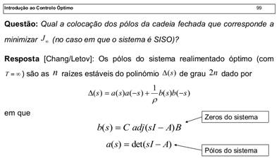
% method 1: pole placement as suggested by Chang-Letov's theorem

sp= 2*exp(j*pi*5/4); % pole value computed in the class

K= acker( A, B, [sp conj(sp)])

% method 1b: pole placement as suggested by Chang-Letov's theorem

sp= roots([1 0 0 0 16]); sp= sp( real(sp)<0 );

K= acker(A, B, sp )

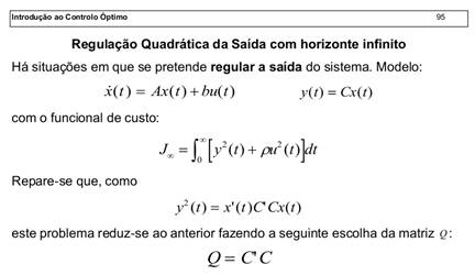
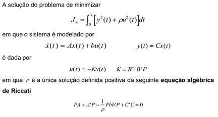
% method 2: formulation as a Linear Quadratic Regulator (LQR):

Q= C'*C;

R= 1/16;

K= lqr( A, B, Q, R)

% LQR implies closed loop stability. See it in the poles:

eig(A - B*K)

---- Table of expressions extracted from the collection of self-study problems:

Files to download from Fenix:

PrContrOpt.pdf – 16 exercise problems for self-study (Portuguese)

CEE-SolucoesProbSeleccionadosContrOptimo.pdf – solutions for various self-study problems

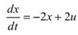
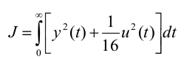
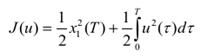
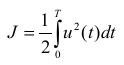
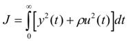
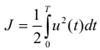
Problem number	System and initial conditions	Merit or Cost function (J)	Bounded or Unbounded control
P1
P2
P3
P4	x(0)=10, x(T)=20, T=1
P5
P6
P7
P8
P9
P10
P11
P12