Linear and Nonlinear State-Space Control Theory
Using
Matlab to explore more the practice-class problems
J. Gaspar
The problems here referred are from the
collection made by Professor João Miranda Lemos
https://fenix.tecnico.ulisboa.pt/downloadFile/1970943312271265/PrCEE-AulasPraticas.pdf
Note1: This page is not the solution
of the exercises (yes, you still need to attend the practice-classes of the
course). This page is in essence a collection of extra information or
simulations obtained / helped by the use of Matlab. Notes2: The control toolbox
is necessary for most of the examples shown bellow. In order to overview the
control toolbox just type in the Matlab prompt the command doc control
P1.
Simulation of a two capacitors circuit using the state space model.
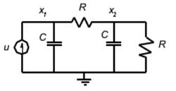
In these simulations R=1KOhm and
C=1mF. Alternative models are generated using random changes of basis. Download
the simulation files p1.m
and p1b.m.
To run the simulation files open the files with Matlab and press F5 or type
their names in the command line (assuming you are in the right folder).
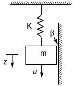
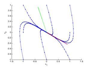
P2. Mass-spring-damper
system
Phase portrait, initial guesses
using just the dynamics matrix: download p2c.mdl,
p2c_tst0.m
and p2c_tst1.m
. For a partial demo run tst0. Run tst1 for the complete demo. These demos
require also Simulink.
P4.
Conversion between models: transfer function to state-space. In Matlab (control
toolbox) you can do simply [A,B,C,D] = tf2ss(num, den)
Challenge: write your own Matlab
function that converts a transfer function to a state space model. Conversion
in the simplest case where the degree of the numerator is lower than the degree
of the denominator can be seen in my_tf2ss.m
and tested by running that function without arguments.
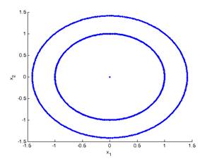
P5.
Mass-Spring-Dumper time response. To see phase space drawings run p5b.m,
where two cases are considered, namely having or not having damping.
P6.
Obtaining transition matrices for systems can be based in the inverse ![]()
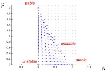
P11. The two
populations cannot coexist. See p11_tst.m.
Depending on the initial conditions, one of the populations is going to
disappear. In the next table (N0,P0) denote equilibrium
points:
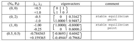
Notice that stable points are (0,2)
and (1,0), so there is no option of (a,b) with a and b simultaneously not zero.
Graphically, local directions show
convergence towards the extinction of one or the other population: