Schneider P57 PLC Memory Analyze
Log Data in the PLC + Analysis with Matlab
2014, 2017, 2019, José Gaspar
Introduction
In this page you can find a method to save data in the memory of a Schneider PLC, namely the TSX Premium P57, then save the data to a file and plot the results using Matlab. This tool has been developed to help debugging PLC programs developed by students in the Industrial Automation course.
Debugging PLC programs involves monitoring inputs and outputs. Provided a PLC program leaves free some memory the resources and allows some more processing time, using the memory for logging inputs and outputs is an appealing solution as one does not need external hardware and therefore have lower costs.
Using PLC memory for logging in many cases is not straightforward. For example, the Schneider Premium PLCs used in our course have proprietary memory map. The memory map actually depends on the programming and therefore cannot be predicted beforehand. The proposal in this page is that by putting some markers in the memory which is dumped to a file, allows using another program (Matlab) to find the logged data, by retrieving the markers.
Preliminary Experiment
In this experiment is used the PLC TSX P57 1634M 02.00 (and DMY28FK, not used in this project). The PLC program, provided in the zip file (see below) fills 501 PLC words, %MW0 till %MW500, with values from zero till 500. After filling this memory map, it can be saved to a file, and then Matlab is used to plot it.
The procedure is the following:
- In case you are using Unity Pro v13 download the zip file data_dump_exp_up13.zip. In case you are using an older Unity Pro (v6), download the zip file data_dump_exp.zip. Decompress the downloaded zip file to a folder of your choice.
- Using Unity Pro, open the file data_dump.stu, transfer the code to the PLC, run the code in the PLC or the PLC simulator.
- Still using Unity Pro, export the memory to a file, PLC -> "Save data from PLC to file". Save data into two files, "mem_dump.dat" and "mem_dump.dtx".
- Using Matlab change to the folder containing the files "mem_dump.dat" and "mem_dump.dtx".
- Within Matlab run: >> mem_dump_load
Following the sequence of commands, Matlab shows two plots with some peaks. Zooming the plots allows retrieving the ramps 0:500. Despite the differences of the DAT and the data extended (DTX) files, you find that both memory maps consist of integer values (16bits), and that the ramps 0:500 are immediately readable.
Data Logger
In this experiment is used also the PLC TSX P57 1634M 02.00, but now with the modules DEY16D2 and DSY16T2 in the slots 2 and 4, respectively. In the PLC program, provided in the zip file (see below), three words are used to mark the beginning and length of the memory area used for logging. The PLC program will then save changes and times of changes of the inputs. In the next section are given more details about the PLC program.
Procedure to test the program:
- In case you are using Unity Pro v13 download the zip file data_log_up13.zip. In case you are using an older Unity Pro (v6), download the zip file data_log.zip. Decompress the downloaded zip file to a folder of your choice.
- Using Unity Pro, open the file data_log2.stu, transfer the code to the PLC, run the code in the PLC or the PLC simulator.
- Change the states of the inputs a number of times (the program is going to save 10 changes). Using the real PLC you can apply voltages to the inputs. Using the PLC simulator, you can force values of the inputs by right clicking on top of the variables %i0.2.x.
- Still using Unity Pro, export the memory to a file, PLC -> "Save data from PLC to file". Save data into the file "data_log2_tmp.dtx".
- Using Matlab change to the folder containing the files "data_log2_tmp.dtx".
- Within Matlab run: >> mem_dump_load_tst
Note, the zip file contains already one file "data_log2_tmp.dtx" and therefore you can start running mem_dump_load_tst.m just to see the plots (these plots are also shown bellow).
Data Logger Description
Figure1 shows the PLC program (the basic configuration of the PLC is not shown in this webpage - you can use Unity Pro to see the configuration). The first IF runs once after loading the program to the PLC and starting to run the program. This IF fills three words marking the start of the memory area to hold the data logging. In particular the word %MW99 has the value 2010 which indicates that 20 memory words, %MW100 till %MW119, are going to hold a matrix with 2 lines and 10 columns (the first digit indicates the number of lines and the next three digits indicate the number of columns).
The section reading the input signals, %i0.2.0 till %i0.2.15, joins all the 16 bits into a single word, namely "acc", and if that word is different from the previous one, it is saved into memory. Together with the input data it is also saved the time encoded as the number of scan cycles.
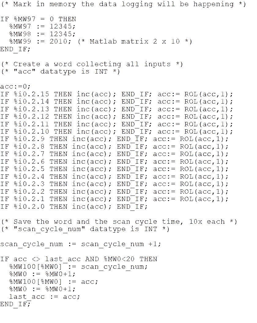
Figure1: PLC sample code to fill memory with events. Using the procedure explained before, these events can be analyzed in Matlab.
Table1 shows a sequence of input changes (this data can be found in file "data_log2_tmp.dtx"). For example, table1 shows that at scan cycle number 902, input bit %i0.2.0 changed from zero to one, and at scan cycle number 1106 it is bit %i0.2.4 that changes from zero to one.
|
Time represented by |
16 input bits represented |
16 input bits represented |
|
902 1106 1300 1522 1901 2101 2307 2483 2812 3132 |
1 17 529 33297 37393 4625 529 17 1 0 |
0000000000000001 0000000000010001 0000001000010001 1000001000010001 1001001000010001 0001001000010001 0000001000010001 0000000000010001 0000000000000001 0000000000000000 |
Table1:
Recorded data. The first column describes time (in number of scan cycles).
The second and third columns show input states in decimal and binary notations.
Figure2 is a graphical representation of Table1, i.e. shows also a sequence of input changes listed in file "data_log2_tmp.dtx". In this case, the display is of the decimal values. Note that this is a simple display created just for illustration - most likely you will want to make separate plots for all the 16 bits.
|
|
|
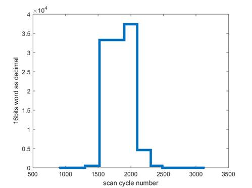
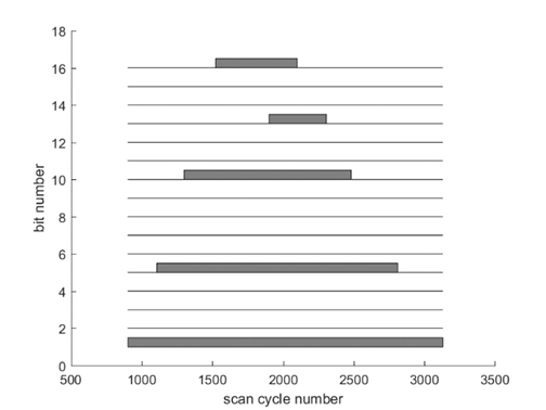
Figure2: The 16 bit inputs form 16 bits words which can be shown in a time plot using decimal notation using simply the stairs Matlab command (left). A better display is to show the bits separately so that low order bits are also visible (right). The plot of the time plots separated per bit has been made with plot_z.m included in data_log.zip .
In the code just described, we are logging just inputs. It is also possible to log output bits. Figure3 shows a program similar to the one in Figure1, but now there is generated a 10Hz square wave to the output bit %q0.4.0. The level transitions of the square wave are logged into a 2x100 buffer. Note that here we are saving one bit into a 16bits word, hence wasting memory. The 16 bits of a word can be completed filled with inputs and outputs (Figure1 was filling all with inputs). Saving of time may also be not necessary in some cases. For example, one may wait for an event on an input bit and after that event save the inputs and outputs at every scan cycle.
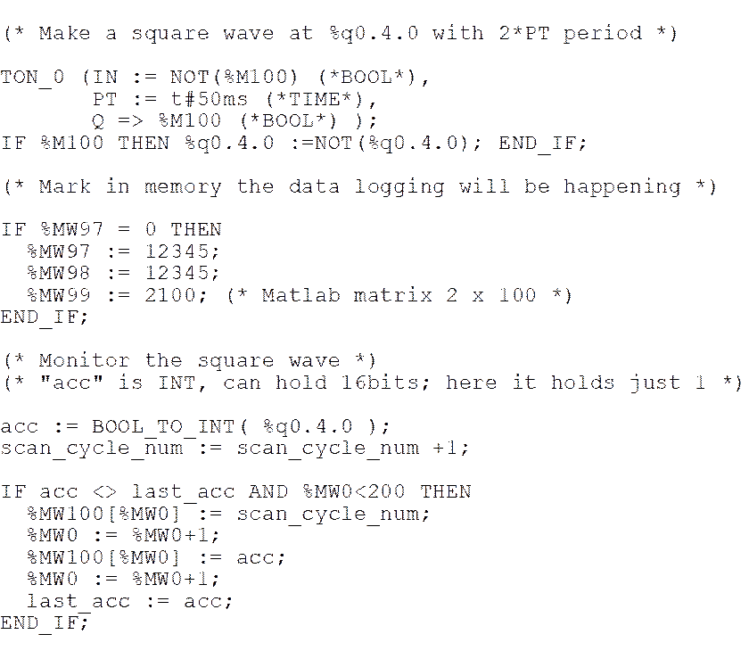
Figure3: PLC code generating a square wave and saving to memory the transition scan-cycle numbers.
Maintenance
This software was created for the purpose of being used in classes. There is no continuous maintenance other than the requirements associated to the classes.
This program is distributed in the hope that it will be useful, but without any warranty; without even the implied warranty of merchantability or fitness for a particular purpose.
Acknowledgment
In case you find this software useful and do any publication in the sequel
please refer to the course Industrial
Automation at Instituto Superior Técnico,
Contact
|
Prof. José Gaspar Instituto de Sistemas e Robótica, Instituto Superior Técnico, Torre Norte Av. Rovisco Pais, 1 1049-001 |
Office: Torre Norte do IST, 7.19 |