Chaining RC Responses: Learning with PSPICE and Matlab/Octave
October 2008, José Gaspar
Main
objectives of this page:
- Building
an analytical expression for the response of a first order circuit (RC series)
given a step voltage source. Using the fact that the form of the expression is
well known, one just needs to find (i) the time constant t, (ii) the initial voltage vc(0), and
(iii) the voltage after infinite time
vc(inf), for
each step in the voltage source.
- Using the
continuity of the capacitor's voltage
to chain several analytical expressions (responses), considering that the
voltage source changes its value from time to time.
|
|
|
|
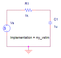
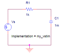
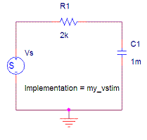
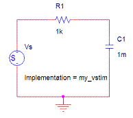
Fig.1 The RC series
circuit, having three different time constants: (left) 1KOhm Resistor and 1
micro Farad Capacitor, (middle) 1KOhm Resistor and 1 mili
Farad (1mF) Capacitor, (right) 2KOhm Resistor and 1mF Capacitor. The voltage
source value along time is encoded in a data file under the label "my_vstim".
Given the
resistance and capacity values of a RC circuit, the time constant, t is immediately determined. For example t=1KOhm*1mF=1ms. The general shape of response
to a constant source voltage is given by:
 (Eq.1)
For
instance, if the capacitor starts discharged and the voltage source changes
from 0V to 5V at t=0s, then the capacitor's voltage along time is simply:
![]() (Eq.2)
(Eq.2)
In case the
voltage source changes its value at various moments, than the response shown in
the previous equations, needs to be adapted accordingly to the changes of the
source. Each step of the source motivates one response, the various responses
have to be "chained" guaranteeing that the final value of one
response is equal to the initial value of the next response.
For
instance, if the voltage source is 0V for t<0ms, 5V for t in [0ms..5ms], and gets to 6V for t in [5ms..10ms],
then the capacitor charges to 5V till t=5ms and then charges a little more,
till 6V, for t=10ms. Then you would have two parts for the capacitors voltage:
 (Eq.3)
In general,
whenever there is a change of the source, a new RC response must be computed,
considering the state where the capacitor was left with the previous source
value.
Lets say
that the voltage source changes at the times t=t00, t10,
t20, ... ti0, then one has to compute the responses v0(t), v1(t), v2(t), ... vi(t),
considering the states where the capacitor was left in the previous step, vi-1(ti0)
and the values to where the capacitor will run, vi(inf) if the current source value remains till infinity. In
summary, the chaining rule is:
 (Eq.4)
1. Simulation of the RC circuit
In this section
we assume that you have installed: (i) the circuit
simulator PSPICE (the student version 9.1 is freeware), and (ii) a matrices
computations tool as Matlab (commercial product) or Octave (freeware; 52Mb for octave-3.0.1 windows
binary).
The
simulation of the circuit and visualization of the results is as follows:
a)
Uncompress to a folder the next file (click to download):
b) Open the
file "rc_resp.opj" with the program Capture
included in PSPICE
c) Simulate
the circuit in the Capture's menu "pspice ->
run" or click in the icon named "Run pspice".
Before starting the simulation, make sure that the window which is selected is
the project's window (".opj") and not the
circuit window.
d)
Visualization of the response using Matlab or Octave:
>> cd c:\directory\where\the\zip\was\decompressed
>> rc_resp_show
e) Choosing
other stimulus (source) signals, can be done also in Matlab
/ Octave:
>> rc_choose_vs(1); % alternatively to 1,
there are also 2, 3 and other choices you can see by editing rc_choose_vs.m
f) After
choosing other stimulus, run again (c) and (d).
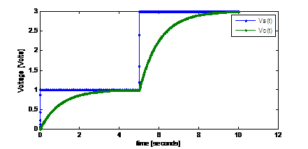
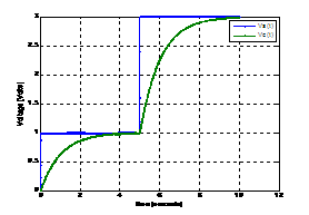
Fig.2 Example of an RC-series response to two steps
displayed with Matlab. In this example tau=1second.
2. Plotting tool to help checking the chained
responses obtained analytically
The
analytical response of an RC-series circuit is obtained simply by filling the
constants in Eq.4, assuming that the source signals are described by
rectangular pulses (sequences of steps). In other words, one just has to find (i) the time constant of the circuit, (ii) the times where
the source changes, and (iii) the voltage values of the source. In this section
we show how to use the "rc_resp_guess"
function to compare the graphics of PSPICE simulations with the analytical
derivations.
Example of
a novel source signal composed by two rectangular pulses, 1[V] and 3[V],
changing at t=5s:
>> rc_choose_vs(1)
Runing as
before the simulation with PSPICE, one obtains the response graphic with:
>> rc_resp_show
Guessing
the response involves inputting a number of values:
>> rc_resp_guess('2step')
-- input first pulse response:
start time
[sec] = 0
tau [sec] = 1
Vc(t=ini) [Volt] = 0
Vc(t=inf) [Volt] = 1
-- input second pulse response:
start time
[sec] = 5
tau [sec] = 1
Vc(t=ini) [Volt] = 1
Vc(t=inf)
[Volt] = 3
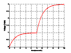
The result
of the previous input of data is a graphic that is superimposed on the active figure
(if you do not want the overlapped graphics, just create a new figure: >>
figure). See Fig.3.
|
|
|
|
Fig.3 RC-series circuit, PSPICE response and
user guess of the response.
3. Further testing
Making short
charging or discharging cycles, e.g. cycles during just one time constant,
makes more challenging the derivation of the analytic responses, since in these
cases the capacitor never gets close to the steady state. Computing the values
at the end of each charge / discharge is therefore necessary to complete the
chaining of the RC responses.
The
function rc_choose_vs helps these kind
of tests by allowing to define interactively source signals having 2
rectangular-pulses or 3 rectangular-pulses. For example defining two pulses
with 3V and 0.5V amplitudes, changing at t=1sec, is done interactively as:
>> rc_choose_vs('2step')
-- input values to define two pulses
(0..t1 and t1..10s)
t1=1
Vs(0..t1)=2
Vs(t1..10s)=3
Similarly
for 3 rectangular-pulses
>> rc_choose_vs('3step')
-- input values to define three
pulses (0..t1, t1..t2 and
t2..10s)
t1=2
t2=3
Vs(0..t1)=5
Vs(t1..t2)=2
Vs(t2..10s)=4
Alternatively,
one can write single command with all the information:
>> rc_choose_vs('2step', [1 3 0.5])
>> rc_choose_vs('3step',[2 3 5 2 4])
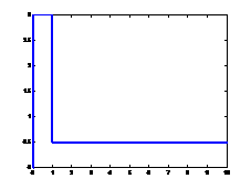
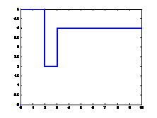
In case you
just want to display the signal before outputting it to PSPICE, you can add a
configuration structure, and obtain the results shown in Fig.4:
>> rc_choose_vs('2step', [1 3 0.5] , struct('sh_signal',[]))
>> rc_choose_vs('3step',[2 3 5 2 4] , struct('sh_signal',[]))
|
|
|
Fig.4 Two source signals, composed
by two or three rectangular-pulses, shown by the rc_choose_vs
function.
Testing the
analytical RC-responses can be done once more using
>> rc_resp_guess('2step')
>> rc_resp_guess('3step')
Alternatively,
the rc_*.m functions include also a basic simulator
of the response, freeing from the need of running the experiments using PSPICE.
Note that in particular the simulator only handles rectangular pulses, and is
therefore not an option to simulate general piecewise linear signals as PSPICE.
The syntax to ask for a simulation is compactly packed into a configuration
structure (note the extra 's' in the string "sh_signals"):
>> rc_choose_vs('3step',[2 3 5 2 4],struct('sh_signals',[]))
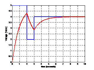
Fig.5 A simulation result for three
rectangular-pulses.
Note: in
case some equations become to hard to read, click here to see these page in PDF.
